Quick Start Guide

Table of Contents

• Setting up
• Classes
• Robochameleon classes
• Signal representation
  • Power representation (pwr)
  • Other signal properties (signal_interface)
  • Relationship between power and waveform
• Block-based program structure (units & modules)
  • Units (unit)
  • Modules (module)
• Accessing constants
• Utility functions
• Examples
• Useful references

Introduction to framework

Overview

Robochameleon is a coding framework and component library for simulation and experimental analysis of optical communication systems. This is a quick start guide to using the framework; descriptions of components can be found in the corresponding class definitions.

We use classes to ensure standardization for both signal representation and functions. This guide has a brief introduction to classes, but if you are familiar with object oriented programming, you should skip it.

Setting up

The Robochameleon project is stored in multiple folders, which all must be in Matlab's search path for the code to run. The script robochameleon.m will automatically add these to the path.

There are also some toolbox dependencies, as well as some function calls to relatively new features in Matlab. When possible, we have added alternatives in the compatibility folder. The initialization script does some automatic detection of what features the user has, but is not perfect, and in some cases it might be necessary to add these folders manually. In particular, [module] uses the bioinformatics toolbox, so the folder \compatibility\bioinfolite should be in the path if the user does not have a license.

Classes

Classes ensure standardization for a large function library. They facilitate block data processing and internal state saving. For a complete introduction to classes using Matlab, there are some useful tutorials on Matlab Central.

Here is a very simple (and totally useless) example of a class that adds two numbers together:

classdef Adder

    properties
        a;
        b;
        sum;
     end
    
    methods
        function obj = Adder(param)
            obj.a = param.a;
            obj.b = param.b;            
        end
        
        function obj = plus(obj)
             obj.sum = obj.a+obj.b
        end
    end
end

A class basically consists of two things:

1. Properties. These are analogous to parameters passed to a function.
2. Methods. These are analogous to functions.

All classes must have a method (called the constructor) that creates an object of that class. In the above example, that was:

function obj = Adder(param)
    obj.a = param.a;
    obj.b = param.b;            
end

In the above example, there is an additional method called plus that contains the main function. To use this class, one would first make an adder using the constructor:

>> test=Adder(struct('a', 1, 'b', 3));
>> test
test = 
  Adder
  Properties:
    a: 1
    b: 3
    sum: []
  Methods

Note the addition has not been performed yet. Then to perform the pre-defined operation:

>> test.plus
ans = 
  Adder
  Properties:
    a: 1
    b: 3
    sum: 4
  Methods

Note all other operations are prohibited:

>> test.minus
No appropriate method, property, or field minus for class adder.

Robochameleon classes

In Robochameleon, there are four basic classes:

1. pwr for representing signal power
2. signal_interface for representing a waveform
3. unit for representing an element in a communication system
4. module a collection of units, including connections between them

Clicking the above links will take you to the full reference pages for each class with documentation of all properties and methods. Below, we have a more general introduction to the most important properties and methods, as well as descriptions of how these are meant to interact.

Signal representation

Signals are described using two classes, pwr, and signal_interface. Each signal_interface object has a property (signal_interface::PCol) that is an array of pwr objects. An array is used so that one pwr object describes the power contained in each each component (polarization) of the waveform.

Power representation (pwr)

Typically signal power is represented as an object of type pwr. The two main properties are

1. the signal-to-noise ratio, and
2. the signal power.

Note that the SNR is not always well-defined (e.g. this value doesn't mean much after propagation through a nonlinear channel). The primary purpose of tracking SNR is to help understand what limits performance of a simulated system, but sometimes some discretion in interpreting this value is required.

The signal power and noise powers are defined as the total powers in the bandwidth of the signal waveform (i.e. the sampling rate Fs). Thus if a large oversampling ratio (e.g. 16 samples per symbol) is used, then the SNR of the signal will be much worse than the SNR of an equivalent signal in a real system.

There are a number of useful methods in the pwr class, including addition, scalar multiplication, and several display and unit conversion functions. These are documented in the class itself. For an example of how to use pwr objects, consult run_Testpwr.m in \Setups\Demo.

Other signal properties (signal_interface)

All signals must be represented as objects of type signal_interface. They have the following user-specified properties:

1. E, the waveform (in arbitrary units)
2. Fs, the sampling rate (Hz)
3. Fc, the carrier frequency (Hz)
4. Rs, the symbol rate (Hz)
5. PCol, the signal power (array of pwr objects)

These quantites are also not always well-defined (e.g. the output of a laser has no symbol rate), but are nonetheless required. signal_interface objects also have some derived properties:

1. N number of signal elements (polarizations)
2. Nss number of samples per symbol
3. ...

which can be read and used but not modified.

Here is a very simple example of how to construct a signal interface object and what the display function looks like:

>> sig_param = struct('Rs',10e9,'Fs',40e9,'Fc',const.c/1550e-9, 'PCol', [pwr(inf, 27), pwr(inf, 27)]);
>> sig_mat = randn(100,2); % 2-component random signal
>> sig_obj = signal_interface(sig_mat,sig_param)

Real signal
              Length: 100 Sa
Number of components: 2
         Symbol rate: 10.0 GBd (100.0 ps)
       Sampling rate: 40.00 GHz (25.00 ps)
  Oversampling ratio: 4.00 Sa/symbol
   Carrier frequency: 193.414 THz (1.55000 um)

Total power: 30.03 dBm (1006.49 mW)
SNR: Inf dB (Inf)
Signal power: 30.03 dBm (1006.49 mW)
Noise power: -Inf dBm (0.00 mW)
>>

There are a number of useful methods in signal_interface that are documented there. Most notably, there are methods to apply functions to signals and add signals to each other such that power and SNR are tracked automatically.

Relationship between power and waveform

Note that the waveform amplitude (signal_interface::PCol) is specified separately from the waveform shape (signal_interface::E). This can lead to un-intended results when the two are in conflict. It is important to always use the appropriate get and set-like (signal_interface::fun1, signal_interface::plus, signal_interface::mtimes) methods when manipulating waveforms.

For an extended example, see run_TestSignalInterface.m and run_TestSignalInterfaceAdvanced.m in \Setups\Demo

Block-based program structure (units & modules)

Every function that can be applied to a signal_interface object is encapsulated in a unit. Multiple units can be collected into a super-unit, which is called a module.

Units (unit)

Everything that operates on a signal_interface object should be defined as a class that inherits certain properties from [unit]. For example:

classdef MyClass_v1 < unit
...
end

All units must have the following properties:

• nInputs
  • Number of inputs
• nOutputs
  • Number of ouputs

Units must also have the following method (in addition to the constructor):

• traverse

Traverse acts like main in c programs. It defines what function the unit performs on the signal. The only allowable inputs and outputs of traverse are of type signal_interface. This is necessary to ensure cross- compatibility between units written by different people, as well as module construction. Everything else should be an object property.

There are a number of properties automatically included in all units. The ones relevant to the user are:

• draw
  • This should be used to enable/disable plotting (true=plot)
• results
  • This is a structure that should be used to store information calculated/gathered by the unit during traverse. Using a general structure for this task is sometimes more convenient than using object properties.

Modules (module)

A module is a collection of connected units. Modules can contain other modules.

A module definition will only have a constructor. The constructor has three parts:

1. A series of constructors for constituent units
2. A series of connections between units
3. The command exportModule

For example:

classdef MyModule_v1 < module
    
    properties
        nInputs = 2;
        nOutputs = 4;
    end
    
    methods
        function obj = MyModule_v1(param)
            % Units
            a = A(param.paramA);
            b = B(param.paramB);
            c = C(param.paramC);
            d = D(param.paramD);
            
            % Connections
            obj.connectInputs({a b},[1 1])
            a.connectOutputs(c,1);
            b.connectOutputs(c,2);
            c.connectOutputs({d obj.outputBuffer obj.outputBuffer},[1 3 4])
            d.connectOutputs({obj.outputBuffer obj.outputBuffer},[1 2]);
            
            obj.exportModule();
        end
    end
    
end

creates a module with the following connection diagram:

Module example

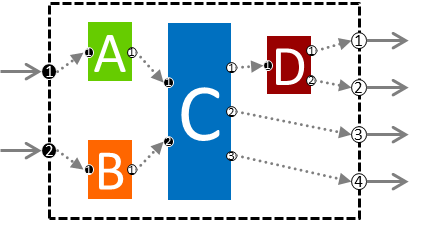
A module is itself a unit. Enabling unit::draw for a module will plot a system diagram (biograph) when the constructor is called. These do not close with close all , but can be removed with close_biographs .

Accessing constants

There is an additional class in base called const where physical constants in standard SI units are stored.

For example, to use the speed of light, enter const.c .

Utility functions

Here is a partial list of generally useful functions:

For creating & programming new units and modules:

Name	Description
createRoboUnit.m	Create a unit using template
increaseClassVersion.m	Create new version of a unit
unit::setparams	Set default parameters in class constructor (replaces paramdefault.m)
robolog.m	Robochameleon log utility (for errors, warnings, etc.)

For running scripts and browsing results

Name	Description
robochameleon.m	Add all robochameleon directories to path
clearall.m	Clear workspace variables preserving breakpoints
close_biographs.m	Close biographs (module diagrams)
findUnit.m	Find a unit within a module (requires full unit name, recursive search)
compileMex.m	Compile all MEX files in project

See also

Robochameleon utilities

Examples

There are a number of examples in the folder. These are organized in order of increasing complexity in numbered sub-folders.

Useful references

For a general overview of the physical layer, the following references may be useful:

1. G.P. Agrawal, "Fiber-Optic Communication Systems", Wiley Series in Microwave and Optical Engineering, John Wiley & Sons, Inc., New York, 2010.

For a general overview of the DSP, we recommend the following papers:

1. S. Savory, "Digital Coherent Optical Receivers: Algorithms and Subsystems," IEEE Journal of Selected Topics in Quantum Electronics, vol. 15, no. 5 (2010).
2. P. Winzer et al., "Spectrally Efficient Long-Haul Optical Networking Using 112/Gb/s Polarization-Multiplexed 16-QAM," Journal of Lightwave Technology vol, 28, no. 4 (2010).
3. K. Kikuchi, "Coherent Optical Communications: Historical Perspectives and Future Directions," in High Spectral Density Optical Communicataion Technologies ed. Nakazawa et al. (Springer 2010).